Manual vs. Automated Smashing

When compressing a model with Pruna, you can manually configure everything or let the Optimization Agent do the heavy lifting. Here's how the two approaches compare:

Manual Smashing

In manual mode, you define your compression setup by specifying which algorithms to use and how to tune their hyperparameters. This approach gives you complete control, but also requires deep knowledge of:

• How each compression technique works

• How to set optimal hyperparameters for your use case

This method best suits expert ML engineers who want fine-grained control over their optimization process.

smash_config = SmashConfig()
smash_config["cacher"] = "flux_caching" # configure the compression configuration
smashed_model = smash(model=base_model, smash_config=smash_config)

⚠️ In this example, you might think using a single cacher is enough, but you could miss out on more powerful combinations of techniques that significantly improve performance when used together.

Automated Smashing

# Load the base model
base_model = FluxPipeline.from_pretrained("black-forest-labs/FLUX.1-dev", **loading_kwargs)

# Define the task
task = Task([
    "psnr", # Quality evaluation
    "elapsed_time", # Speed evaluation
], 
datamodule=datamodule)  # configure the metrics of interest for this use case

# Start the optimization agent
optimization_agent = OptimizationAgent(model=base_model, task=task)
smashed_model = optimization_agent.probabilistic_search(n_trials=10)

Compression can get complex fast — the configuration space is exponentially ample, and the best setup depends on:

1. Your model architecture

2. The target hardware

3. Your optimization objectives (e.g., quality, latency, memory)

That’s where the Optimization Agent comes in. It automates the process by:

• Detecting compatible compression techniques for your model and hardware

• Choosing the best combinations of algorithms

• Tuning hyperparameters based on your objectives

All you need to do is:

1. Load your base model

2. Define the task (which includes your evaluation metrics)

3. Launch the optimization

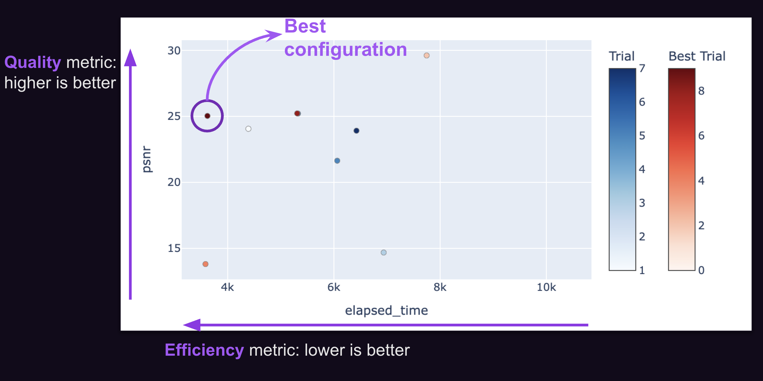
Reviewing the Results

Once the optimization is complete, you can visualize the results using a Pareto front plot, which shows all trade-offs between speed, quality, and memory. Pick the best configuration for your needs. Voilà!